ccvmplotlib#
ccvmplotlib#
ccvmplotlib contains code for plotting results from the ccvm package. It extends Matplotlib to generate visualizations for various problem classes supported by the CCVM architecture.
Features#
Class Diagram#
The diagram provides more details in how plotter library can be used and the asscoatiated class relationship.

Usage#
from ccvmplotlib import ccvmplotlib
METADATA_FILEPATH = "./tests/metadata/valid_metadata.json"
PLOT_OUTPUT_DEST = "./"
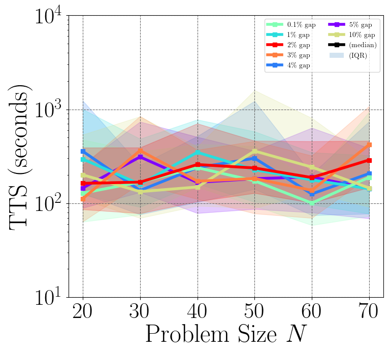
# Generate TTS plot
tts_plot_fig, tts_plot_ax = ccvmplotlib.plot_TTS(
metadata_filepath=METADATA_FILEPATH,
problem="BoxQP",
TTS_type="wallclock",
)
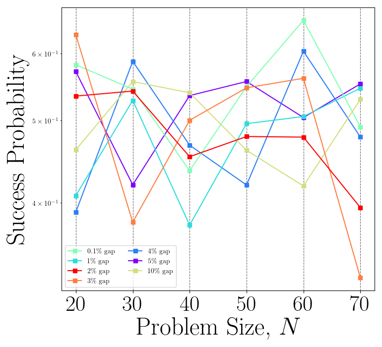
# Generate success probability plot
succ_prob_plot_fig, succ_prob_plot_ax = ccvmplotlib.plot_success_prob(
metadata_filepath=METADATA_FILEPATH,
problem="BoxQP",
TTS_type="wallclock",
)
# Apply default styling
ccvmplotlib.apply_default_tts_styling(tts_plot_fig, tts_plot_ax)
ccvmplotlib.apply_default_succ_prob_styling(succ_prob_plot_fig, succ_prob_plot_ax)
# Save plots
tts_plot_fig.savefig(PLOT_OUTPUT_DEST + "tts_plot_example.png", format="png")
succ_prob_plot_fig.savefig(PLOT_OUTPUT_DEST + "success_prob_plot_example.png", format="png")
Also, a pre-processed figure object and axis object can be passed to the plotting methods.
# ...

plot_fig1, plot_ax1 = plt.subplots()
plot_fig2, plot_ax2 = plt.subplots()
"""
Custom modification on 'plot_fig1' and 'plot_ax1' (e.g. plot_ax1.plot(...))
...
Custom modification on 'plot_fig2' and 'plot_ax2' (e.g. plot_ax2.plot(...))
...
"""

# Generate TTS plot by passing a fig and an ax object
tts_plot_fig, tts_plot_ax = ccvmplotlib.plot_TTS(
    metadata_filepath=METADATA_FILEPATH,
    problem="BoxQP",
    TTS_type="wallclock",
    fig=plot_fig1,
    ax=plot_ax1,
)

# Generate success probability plot by passing a fig and an ax object
succ_prob_plot_fig, succ_prob_plot_ax = ccvmplotlib.plot_success_prob(
    metadata_filepath=METADATA_FILEPATH,
    problem="BoxQP",
    TTS_type="wallclock",
    fig=plot_fig2,
    ax=plot_ax2,
)
Figures#
The plotting methods return a plot figure object and a plot axis object with minimal styling (e.g. plot colors, logagrithmic y-scale, etc.), and this allows users to apply their own styling before saving the figure as a file.


However, a default styling method for each plot is provided and can be used as the example above.